Is soybean use driving global deforestation?

Team 5 Look Alive

library(tidyverse)
library(tidymodels)
library(palmerpenguins)
library(knitr)
library(xaringanthemer)
library(ggdark)
library(scales)
library(viridis)
library(gghighlight)
library(styler)

knitr::opts_chunk$set(echo = T)

ggplot2::theme_set(ggplot2::theme_minimal(base_size = 20))

Introduction

Our data comes originally from the UN Food and Agriculture Organization’s Forest Resources Assessment. “Since year-to-year changes in forest cover can be volatile, the UN FAO provide this annual data averaged over five-year periods.” It measures the area of forests over time in countries around the world. It also holds more detailed information about the loss of Brazilian forest over time. The data further holds data about soybean production and vegetable oil production by year and country.

Thre are 5 datasets we are working with: forest, forest_area, brazil_loss, soybean_use, and vegetable_oil. The set forest contains the change every 5 years in for forest area in conversion. forest_area contains the change in global forest area as a percent of global forest area. brazil_loss contains the loss of Brazilian forest due to specific types of deforestation, such as fire and small_scale_clearing. soybean_use contains the soybean production and use by year and by country. Finally, the set vegetable_oil contains vegetable oil production by crop type and year.

What we want to explore in the following visualizations is which countries are seeing the most deforestation within their borders, and to understand the causes of this deforestation. After initially looking at a line plot and seeing that Brazil has faced notably high levels of deforestation, we will look at the following.

• Brazil’s cumulative forest loss 2000-20113
• Causes of forest loss in Brazil
• Top global consumers of soybeans
• Global soybean use proportions over time
• Total global net forest conversion

What countries are seeing the most deforestation within their borders, and what is causing this deforestation?

Introduction

These ideas stuck us as the most essential elements of deforestation, and gaining an understanding of the complexities of deforestation depends on becoming familiar with these concepts.

Approach

In this question, we planned on exploring three things: the who, the what, and the why of deforestation. First, we chose to use a line plot to examine trends over time in deforestation. This would allow us to get a rough understanding of how many countries are facing the most deforestation and examine the most deforested country’s data, using a cumulative line plot of deforestation and a bar plot to compare across years. From here, we could then examine the “what”. To do this, we decided to compare the proportions with an area plot. This gave us the opportunity to showcase which causes are the most impactful in Brazil’s deforestation. Finally, to understand the “why” of deforestation, we selected to examine one of the leading causes of deforestation in Brazil. Using line plots again allowed us to highlight which regions and countries are most influential in driving soybean production globally.

Putting all of these factors together gives us a basic understanding of global deforestation.

Analysis

Figure 1

# these relabel col 1 but we don't care bc it's meaningless
forest <- read_csv("data/forest.csv")
forest_area <- read_csv("data/forest_area.csv")
brazil_loss <- read_csv("data/brazil_loss.csv")
vegetable_oil <- read_csv("data/vegetable_oil.csv")
soybean_use <- read_csv("data/soybean_use.csv")

brazil_loss <- brazil_loss %>%
  rowwise() %>%
  mutate(total_brazil_forest_loss_hectares = sum(c_across(commercial_crops:small_scale_clearing))) %>%
  ungroup()

annotation <- tibble(
  x = c(2010),
  y = c(-7300000),
  label = c("Brazil has lost")
)
annotation2 <- tibble(
  x = c(2010),
  y = c(-10500000),
  label = c("over 30 million")
)
annotation3 <- tibble(
  x = c(2010),
  y = c(-15700000),
  label = c("hectares of forest\nsince 2000")
)

brazil_loss <- brazil_loss %>%
  select(year, total_brazil_forest_loss_hectares) %>%
  add_row(year = 2000, total_brazil_forest_loss_hectares = 0, .before = 1) %>%
  mutate(cum_sum = -(cumsum(total_brazil_forest_loss_hectares)))

ggplot(brazil_loss) +
  geom_line(aes(year, cum_sum), size = 2, color = "#009739") +
  geom_bar(aes(year, -total_brazil_forest_loss_hectares), stat = "identity") +
  geom_hline(aes(yintercept = 0), color = "black", size = 1.5) +
  labs(title = "Cumulative Brazilian forest loss", subtitle = "2000 to 2013", x = NULL, y = "Hectares", caption = "Fig. 1") +
  scale_y_continuous(labels = label_number_si()) +
  scale_x_continuous() +
  geom_text(
    data = annotation, aes(x = x, y = y, label = label),
    color = "black",
    size = 6, angle = 0
  ) +
  geom_text(
    data = annotation2, aes(x = x, y = y, label = label),
    color = "red",
    size = 7, angle = 0, fontface = "bold"
  ) +
  geom_text(
    data = annotation3, aes(x = x, y = y, label = label),
    color = "black",
    size = 6, angle = 0
  ) +
  scale_x_continuous(breaks = seq(from = 2000, to = 2013, by = 4)) +
  theme(panel.grid.minor.x = element_blank())

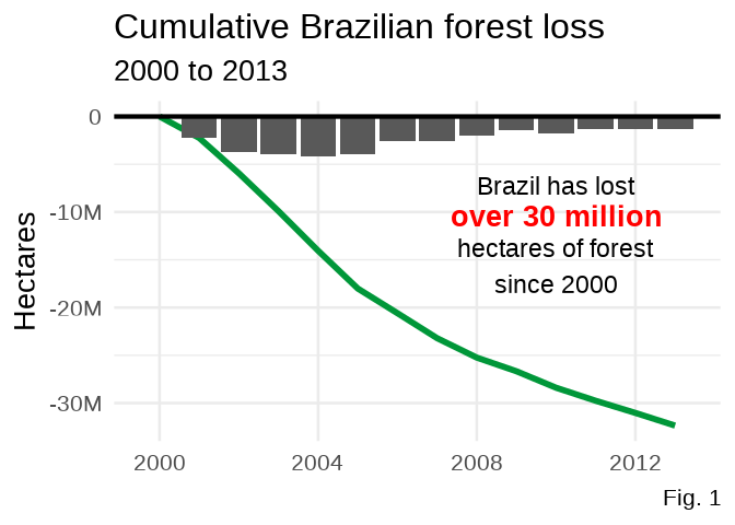
Figure 2

brazil_loss_no_total <- read.csv("data/brazil_loss.csv") %>% select(-(1:3))
brazil_loss_no_total <- brazil_loss_no_total %>%
  pivot_longer(!year,
    names_to = "cause",
    values_to = "forest_lost"
  ) %>%
  mutate(cause = case_when(
    cause == "pasture" ~ "Pasture",
    cause == "fire" ~ "Fire",
    cause == "commercial_crops" ~ "Commercial Crops",
    cause == "selective_logging" ~ "Logging",
    cause == "small_scale_clearing" ~ "Small-Scale Farming",
    T ~ "Other"
  ) %>%
    factor(levels = c("Fire", "Logging", "Small-Scale Farming", "Commercial Crops", "Pasture", "Other"))) %>%
  group_by(cause, year) %>%
  summarise(sum = sum(forest_lost), .groups = "drop") %>%
  group_by(year, cause) %>%
  summarise(n = sum(sum)) %>%
  mutate(percentage = n / sum(n))

ggplot(brazil_loss_no_total, aes(year, percentage, fill = cause)) +
  geom_area(alpha = 0.9) +
  scale_fill_manual(values = c("#6CACE4", "lightgoldenrod", "#EE1C25", "#0A3161", "#009739", "gray")) +
  scale_y_continuous(labels = scales::percent) +
  labs(
    x = NULL, y = NULL, title = "Causes of loss of forest in Brazil", fill = NULL,
    caption = "Fig. 2"
  ) +
  scale_x_continuous(breaks = seq(from = 2000, to = 2013, by = 4)) +
  theme(legend.position = "bottom") +
  guides(fill = guide_legend(override.aes = list(size = 0.3)))

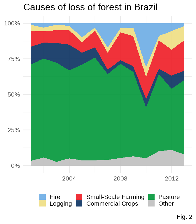
Figure 3

soy_use_by_country <- soybean_use %>%
  filter(
    !is.na(code),
    entity != "World"
  ) %>%
  rowwise() %>%
  mutate(total = sum(human_food, animal_feed, processed, na.rm = T))

# https://stackoverflow.com/questions/49438953/selective-labeling-for-ggplot-lines
# https://cran.r-project.org/web/packages/gghighlight/vignettes/gghighlight.html

soy_use_by_country %>%
  ggplot(aes(x = year, y = total, color = entity)) +
  geom_line(show.legend = F, size = 2) +
  gghighlight(max(total),
    max_highlight = 4,
    label_params = list(hjust = -0.3),
    unhighlighted_params = list(
      size = 1.2, colour =
        alpha("gray", 0.6)
    )
  ) +
  scale_y_continuous(labels = label_number_si()) +
  labs(
    y = "Tonnes", x = NULL, title = "Soybean use by country",
    caption = "Fig. 3"
  ) +
  # flagcolorcodes.com
  scale_color_manual(values = c("#6CACE4", "#009739", "#EE1C25", "#0A3161")) +
  scale_x_continuous(
    breaks = seq(from = 1960, to = 2013, by = 10),
    limits = c(1960, 2025)
  )

Discussion

Figure 1 portrays the amount of lost forest in Brazil in the span of 13 years, from 2000 to 2013. The loss is striking at over 30 million hectares (300,000 square km, for reference). The figure does show a concave trend, which shows that the loss of forest is not exponential, signaling that there may be hope in a continued flattening of this line of forest loss. It is interesting to consider what factors may have contributed to these trends within Brazil. Lawmaking and leadership will play a role in a country’s development, meaning that it would be fascinating to gather this same data from Jair Bolsonaro’s current reign as Brazil’s president and compare it to the trends under Brazilian presidents who led during the time period of this plot, such as Lula de Silva, who served as president from 2003-2010 in Brazil (Wikipedia, Brazilian Presidents).

Figure 2 offers a view of the causes of Brazilian loss of forest. The most common reason for removal of forest in Brazil is to clear space for land to be used as pasture. Other big causes of loss of forest include fire, logging, small-scale farming, and commercial crops. Fires fluctuate wildly on the plot, demonstrating their lack of predictability and their destructive nature. Global warming and human activity may be factors that contributes to the increased danger of forest fires in the Amazon (Bush et. al. 2008). One important commercial crop is soybean, which we chose to analyze further, guided by our retrieval of data on soybean use.

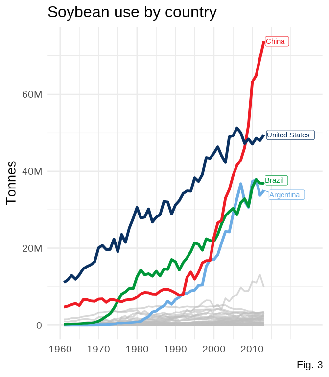
Figure 3 gives a look into which countries are the largest consumers of soybean, which in turn increases demand for soybean and drives deforestation. China, the United States, Brazil, and Argentina were found to be the most prevalent soybean consumers. Argentina was the most surprising to us, but we found that soybean is a vital crop to Argentina, which incentivizes the use of soybean after its growth (croplife, Soybeans in Argentina).

How does the proportions of soybean production used for human food versus for feeding animal change over time? Is this change in proportions related to global deforestation?

Introduction

In the second question, we wanted to start understanding the patterns of soybean use over time. After gaining an understanding of how total soybean use and production have drastically increased around the world in the last 50 years, we looked in question 2 at the specific ways soybean is used within an overall increasing trend and how that relates to deforestation globally.

Approach

In particular, we planned on exploring the proportional changes over time in the share of soybean production used for human consumption compared to its share for feeding animals, and hereby better understand if this change in proportion relates to the aggravation of global deforestation.

First, we chose to use a stacked bar chart to examine changes in production share over time between soybean usage for human food and for animal feed. This would allow us to get a general grasp on whether the overall global increase in soybean production is driven by an added demand in producing human food (i.e. tofu, tempeh, or other dairy substitutions) or a demand increase in feeding livestock (i.e. hogs, poultry, beef). From here, we wanted to see if this proportional change in the share of soybean production has any effect on the rate of global deforestation over time, by using a line plot to represent the rate of change in global net forest conversion.

Putting these two plots together gives us an idea on which sector within the increase in global soybean production might be related with continued forest conversions.

Analysis

Figure 1

use_prop <- soybean_use %>%
  group_by(year) %>%
  summarise(
    total_human = sum(human_food, na.rm = T),
    total_animal = sum(animal_feed, na.rm = T)
  ) %>%
  pivot_longer(!year,
    names_to = "use",
    values_to = "amount"
  )

use_prop <- use_prop %>%
  group_by(year) %>%
  mutate(prop = amount / sum(amount))

use_prop %>%
  filter(year >= 1977) %>%
  ggplot(aes(fill = use, y = prop, x = year)) +
  geom_bar(position = "fill", stat = "identity") +
  scale_x_continuous(
    name = "Year",
    limits = c(1990, 2013),
    breaks = seq(from = 1990, to = 2013, by = 10)
  ) +
  scale_y_continuous(
    name = "Proportion",
    labels = c("0%", "25%", "50%", "75%", "100%")
  ) +
  scale_fill_manual(values = c("#6CACE4", "#009739"),
    name = NULL, labels = c("Animal food", "Human food")
  ) +
  labs(
    title = "Global soybean production and use share between 1961-2013",
    subtitle = "By types of usage",
    caption = "Fig. 4"
  ) +
  theme(
    plot.title = element_text(face = "bold", size = 17),
    plot.subtitle = element_text(size = 15),
    legend.position = "bottom",
    legend.key.size = unit(.5, "cm"),
    legend.text = element_text(size = 12),
    legend.box.spacing = unit(0.2, "cm"),
    axis.title.x = element_text(size = 15),
    axis.title.y = element_text(size = 15),
    axis.text.x = element_text(size = 9, face = "bold"),
    axis.text.y = element_text(margin = margin(t = .3, unit = "cm"), size = 9, face = "bold")
  )

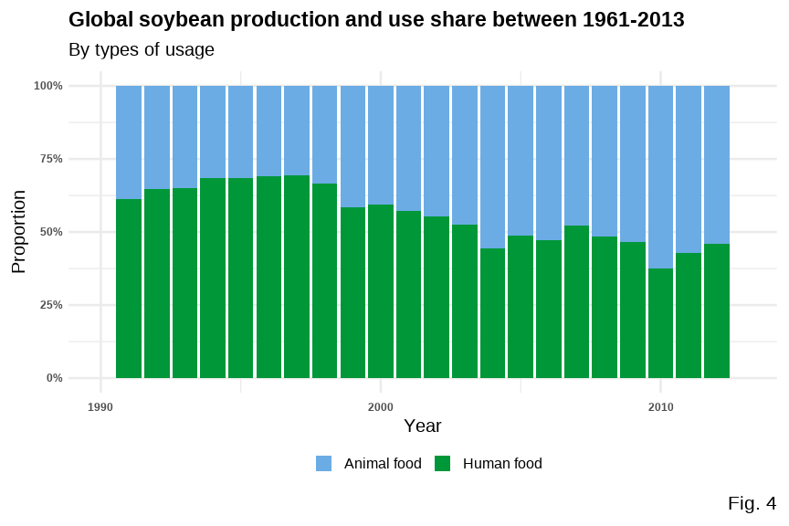
Figure 2

forest2 <- forest %>%
  filter(entity == "World")

ggplot(forest2, aes(x = year, y = net_forest_conversion, fill = year)) +
  geom_area(aes(color = entity), size = 2.5, fill = "lightgray", alpha = 0.5) +
  scale_color_manual(values = c("#009739")) +
  scale_y_continuous(labels = label_number_si()) +
  scale_x_continuous(
    limits = c(1990, 2013),
    breaks = seq(from = 1990, to = 2013, by = 10)
  ) +
  labs(title = "Global Net Forest Conversion (hectares)", x = "Year", y = NULL, caption = "Fig. 5"
  ) +
  theme(
    legend.position = "none",
    plot.title = element_text(face = "bold", size = 17),
    axis.title.x = element_text(size = 16),
    axis.text.x = element_text(size = 13, face = "bold"),
    axis.text.y = element_text(margin = margin(t = .3, unit = "cm"), size = 13, face = "bold")
  )

Discussion

Figure 1 portrays the changing proportion of how much soybean is used for animal feed versus human food each year 1961-2013. We can see a relatively clear trend of an increase in animal/human food use. What we had observed is that the proportion of soybean use for animal feed (mostly used for feeding poultry, hogs, cattle and dairy production ) drastically increased, from less than 10% share in 1961 to more than 50% share in 2013; while the proportion of soybean use for human food (like salad oil, tofu, or tempeh) had decreased accordingly. Soybean meal is a highly palatable form of protein, and is often used as the dominant source of protein for most types farm animals, including pigs, cattle, poultry and aquaculture (Soybean Meal). Knowing this, it was not surprising to see that animal use has increased, as we know that humans as a species are eating more meat.

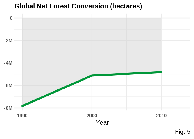
Figure 2 shows the global net forest conversion in hectares (1000 sq m). Net Forest conversion is the clearing of natural forests to use the land for another purpose. Since the net forest conversion are all negative (not positive), from 1990 till 2015, it means that more natural land continues to be used for other purposes, just at a slowing rate. A slowed rate of deforestation is a good thing, but it is not the same as afforestation (turning cleared land back into natural forest).

We might speculate that the increasing proportion of soybean used for animal feed indicates a relationship with increased livestock rearing. Livestock require land, so seeing a continued rate of deforestation with large proportions of soybean use being for livestock makes sense to us. We also see, in the soybean use trend, happening in the late 1990s and early 2000s, with the proportion somewhat evening out in recent years. This matches what we see in global deforestation trends as the rate of global deforestation has slowed.

Overall, we have seen that increased global use of soybeans is related with continued deforestation in Brazil, the world’s leading soybean producer (surpassing USA as of May 2021). And an increased proportion of soybeans used for animal feed (vs. those used for human food) is related with continued land conversion (natural land –> human used), albeit at a slower rate.

Presentation

Our presentation can be found here.

Data

Ritchie, H. and Roser, M. 2021, “Forests and Deforestation”. Published online at OurWorldInData.org. Retrieved from: ‘https://ourworldindata.org/forests-and-deforestation’ on September 13, 2021 [Online Resource]

References

1. Brazilian Presidents
2. Bush, M. B., Silman, M. R., McMichael, C., & Saatchi, S. (2008). Fire, climate change and biodiversity in Amazonia: a Late-Holocene perspective. Philosophical transactions of the Royal Society of London. Series B, Biological sciences, 363(1498), 1795–1802. https://doi.org/10.1098/rstb.2007.0014
3. Soybeans in Argentina
4. Our World in Data
5. Deforestation
6. Share of forest area
7. Drivers of deforestation
8. Deforestation by commodity
9. Soybean production and use
10. Palm oil production 10.Net Forest Conversion
11. Soybean meal